Daniel Koska

Data; Science; Biomechanics

Welcome

This is intended to be a collection of ongoing and past projects, papers, coding adventures and whatever else seems worth sharing. This blog’s running on GitHub Pages and is written using Quarto, (hopefully) making it easy to share code examples. And hey, if you spot something cool, you can dive straight into the GitHub repo and start playing around with it.

Software contributions

Click to expand

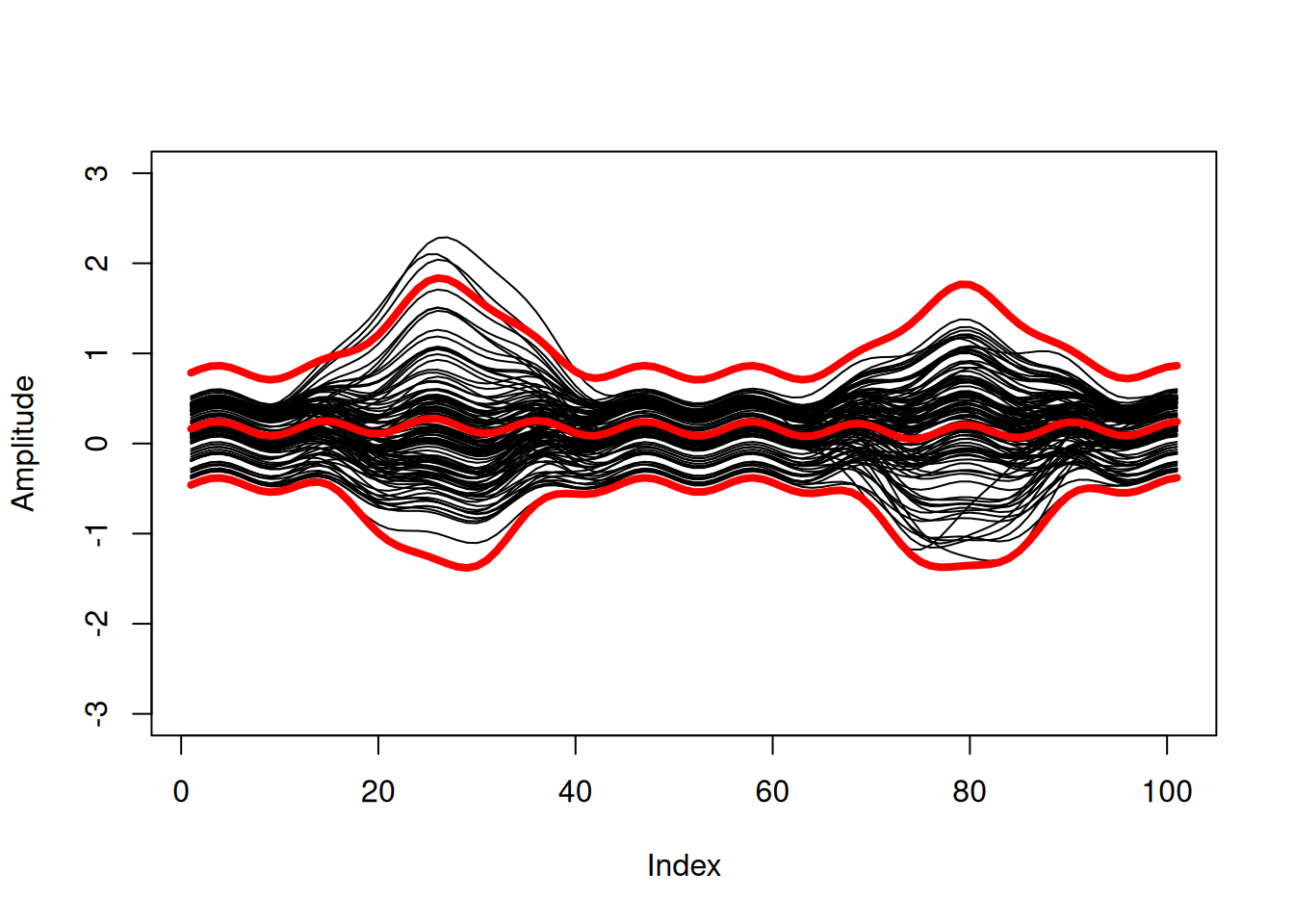
Functional Bootstrapped Bands (FunBootBand)

Background story

Click to expand

The whole journey began when I started thinking about ways to adequately characterize differences between joint angles calculated from different measurement systems. In my case, I wanted to compare joint angles from a 3D camera system and an inertial measurement unit system. In terms of choosing appropriate statistics, there are some good reads about what not to do and how to implement methods for discrete data. See, e. g., the highly cited work by Bland and Altman (e.g the papers form 1986, or 2007), who introduced the so called Limits of Agreement (LoA) approach. There’s much less literature, however, on how to handle continuous differences between two measurement systems.

One paper that caught my attention is the article by Røslien et al., (2012), which describes a way to expand the LoA method to continuous data by using a functional approach. The paper in a nutshell: Continuous data (aka curves) are approximated using functions to calculate a functional counterpart of the LoA. The problem, however, is that the approach described in the paper is not entirely functional. Rather, the actual calculation of the Functional Limits of Agreement is carried out for each individual point of the previously determined functional curves (for details see the implementation in the utilized R package fda by James Ramsay). Strictly speaking, this turns the whole idea of using functions on its head and results in functional LoA (or more generally: statistical bands) that are likely too narrow (Koska et al., 2023). Applied to my original problem of describing continuous differences between measurement systems, this would mean that the random measurement error is likely underestimated.

Another paper that describes a functional approach is the one by Lenhoff et al. (1999), i.e., curves/time series are approximated using functions just like in Røislien et al. (2012). The paper is not specifically about quantifying differences between measurement systems, but more generally about the construction of statistical bands (more precisely confidence and prediction bands) for biomechanical curve data. The actual hack here is that the distribution of curves is estimated by bootstrapping the coefficients of the curve functions. This means that bands are no longer calculated pointwise, but the entire curve is included in the calculation. The method in Lenhoff et al., to the best of my knowledge, is based on the work of Olshen, Biden, Wyatt, and Sutherland from the 1980s (see, for example, Sutherland et al., 1988; Olshen et al., 1989).

Sutherland, D., Olshen, R., Biden, E., Wyatt, M., 1988. Development of Mature Walking. Mac Keith Press. Olshen, R.A., Biden, E.N., Wyatt, M.P., Sutherland, D.H., 1989. Gait analysis and the bootstrap. Ann. Statist. 17 (4), http://dx.doi.org/10.1214/aos/1176347372.
Olshen, R.A., Biden, E.N., Wyatt, M.P., Sutherland, D.H., 1989. Gait analysis and the bootstrap. Ann. Statist. 17 (4), http://dx.doi.org/10.1214/aos/1176347372.

As you can see, the method is not exactly new. I was all the more surprised that I wasn’t able to find a coded version of the algorithm online. This forced me to implement the algorithm from scratch, which I did using R and the formulas in the appendix of Lenhoff et al. (1999). Extremely helpful at this point was the Matlab code that a former colleague at our institute, Dr. Doris Oriwol, kindly provided me with. Her code allowed me to cross-check my implementation and correct a couple of mistakes. For instance - if I remember correctly - I struggled to implement the correction facor that adjusts the width of the bands to the desired confidence level. Not sure if I’d gotten it right without Doris’ help. So, full credit to Doris!

As a side note: I am very grateful for people who have the know-how and the time to review the code. The description in the Lenhoff paper is rather brief, and we were not always 100% sure whether we had correctly implemented the algorithm. Further opinions and possible corrections are very welcome.

I’m sure other researchers have been here before and would have loved to read a coded version of the algorithm. My hope is that sharing our code is a major pain release in that regard and will lead to more people adopting the method. As indicated by Lenhoff et al., functional statistical bands are not limited to the description of differences between measurement systems, but are useful wherever the variation of curve data needs to be analyzed statistically. This includes a ton of important tasks such as estimating population parameters, indicating precision, assessing statistical significance, comparing groups, forecasting future observations, quantifying uncertainty in predictions etc..

In the course of implementing the method, I noticed something else: The examined bootstrap methods (including that of Røislien) have implemented a naive bootstrap, meaning they assume independence of the curves in the dataset. Accordingly, the papers suggested to include only one curve per subject in the bootstrap. From a methodological point of view, this is somewhat problematic since it ignores the intraindividual variance component. In the context of investigating measurement errors, for instance, this means that the variance across repeated measurements within a person is not taken into account. This may further aggravate the problem of bands being too narrow.

We therefore extended the functional bootstrap bands to include a possibility to account for repeated measurements (i.e., dependent curves). This was realized using the two-stage or double bootstrap described in Davison and Hinkley (1997), in which subjects (including all of their curves) are sampled with replacement in the first stage, and one curve per subject is drawn without replacement in the second stage. In addition to sharing our code, this implementation of the two-stage bootstrap is - IMHO - the main contribution of ‘our’ FunBootBand method. A systematic comparison of the method with other methodological approaches for characterizing continuous differences between two measurement systemes (pointwise LoA, Functional LoA, Functional Bootstrapped bands) can be found in in Koska et al. (2023). Here, we analyzed the coverage probabilites of these models in different error scenarios (simulated and real-world data) and found that the FunBootBands showed superior performance.

What follows are various versions of the functional bootstrap bands (ongoing development) in different programming languages. The R code has already been published as a (devtools) package, and I plan to add it to CRAN at some point as well. In addition, I’m currently porting the code to Python. If time permits and I can delve into Julia, this may be next in line. Besides porting the function to different languages to improve the accessibility, my main goal is to increase code efficiency and reduce computation times - after all, bootstrapping is quite a computationally intensive. In R this may be done using RCpp, a C++ version. In Python, there is Cython, which should significantly reduce execution time.

FunBootBand R

Click to expand

The FunBootBand package contains a function to generate statistical (prediction or confidence) bands from curve data using a functional approach and bootstrapping.

The development version of FunBootBand can be installed from GitHub with:

devtools::install_github(“koda86/FunBootBand”)

FunBootBand Python

Click to expand

The first alpha-ish version is available, see here: https://github.com/koda86/FunBootBand-python

My TODO list still includes a bunch of items, such as extensive testing … I’m getting there. Learned a whole lot about Python in the process as well so far.

FunBootBand RCpp

Click to expand

On my TODO list.

Effort to compress

Click to expand

While trying out different complexity measures, I stumbled upon the ‘effort to compress’ (ETC) method introduced in (Nagaraj et al., 2013). ETC is a complexity measure for which code was originally presented as Matlab and Python Code. This repository contains an R implementation of the algorithm.

effort2compress (GitHub)

See also the website of Nithin Nagaraj for the Matlab and Python versions: Website Nagaraj

Python implementation: Github

Identify duplicates in metadata (DupliCheck)

Click to expand

I was recently conducting a meta-analysis to get an idea of the effect of digital physiotherapy for the treatment of various orthopedic diseases. For this, I used Pubmed, Cochrane, BASE (Bielefeld Academic Search Engine) and Embase, which resulted in large csv files containing metadata from the identified scientific articles. This metadata includes paper titles, authors, and the DOI, among others. Not going to talk about the pain of designing adequate search strings and exporting these articles here …

Before deciding which papers to include in the meta-analysis, I needed to identify duplicates, i.e., papers that appeared more than once. This seems like a fairly straightforward job, but, as usual, the devil is in the detail. This probably explains why I wasn’t able to find a suitable R function for the job (though, to be honest, I didn’t invest an awful lot of time searching).

One obvious candidate, the base function duplicated(), only works on exact copies of a string and fails if even a single character is off. This happens, for example, when author names are written differently across databases. For instance, the author “Çelik” is not the same as “Celik.” Another issue is that two distinct papers can have identical titles and the same authors (in a different order). This should be discernible from their different DOIs, but DOIs are not always available and often come in various formats. The list of complications goes on, making the task more complex. To spare others from the same pain, I packed everything into a small R package called DupliCheck.

The package contains a single function called dupliHunter. dupliHunter takes a data frame with (at least) title, author, and DOI columns. It also includes a threshold parameter to possibly fine-tune the allowed similarity between titles (calculated using stringdist::stringdistmatrix with the Jaccard distance method).

Here’s how you can use the package:

library(usethis)
library(devtools)
# devtools::install_github("koda86/DupliCheck")
library(DupliCheck)

load("~/tmp/data.RData") # Example data; load your own data here

duplicates <- dupliHunter(data,
                            title_col = "Title",
                            author_col = "Authors",
                            doi_col = "DOI",
                            threshold = 0.03)

The current version of the function works decently. I haven’t quantified Type I and II error rates so far, but my experience from working with several datasets and the feedback from colleagues suggest that errors are minimal. I’m also optimistic about the function’s ability to generalize across data from different search engines since the tested files represent data from commonly used sources.

Computational cost and execution speed were issues with my initial (simplistic) loop-based approach. I did some optimzation that included preprocessing titles to escape special characters, or the use of parallel processing. This reduced the execution time for a 4191-row test file significantly (down from 2856 s to about 952 s). It’s not lightning fast, but it’s acceptable for vanilla R code. I hope to port the code to C++ to speed up processing time for future projects. We’ll see …

Disco Diffusion Music Video

Click to expand

This post is about a (‘AI’-generated) music video that I created for my Band ICTRL. Before I go on with the nerdy details, you should check out the video first:

The video illustrates our song Dead Horse, which is the first of a bunch of singles we are going to drop this year. The idea to create a video like this was inspired by a Reddit post about a recent video by one of my favorite bands: King Gizzard and the Lizzard Wizard (the song is called Iron Lung). The post provided some insights into how the video was created, e.g. this quote from user No_Stay2400:

“From Spod, the guy who made it (in a Reddit post back when it came out): Cheers, yeah it was 2 months of trial and error, and using a bunch of different techniques alongside the newest diffusion programs as they rolled out. It was all mapped out frame by frame to work with the music, trying see if I could illustrate the feeling of the music through the video. At times it feels like driving a bus from the backseat, but is amazing when it all comes together. The hardest thing is steering it away from the generic look that AI art can get. Anyway, thanks.”

The main tool that caught my interest was Disco Diffusion, a neat open-source AI tool for generative art. Imagine typing in some text prompt and getting intricate pieces of visual art (for all “future” readers of the last sentence: Imagine a world where ‘AI’ was a new and exciting thing). Quickly, the idea was born to create a low-budget video where the prompts and thus the video sequences fit the lyrics of the song.

Disco Diffusion was developed using Google Colab, which is a free, cloud-based Jupyter notebook environment provided by Google. If you are a data scientist or machine learning practitioner, you have probably heard of it. Being cloud-based, Colab requires no setup or installation. Users can start coding immediately in their web browser. Colab supports Python, so it was easy to read and understand the code. That bein said, there’s absolutely no need for any programming skills, since there are empty fields for all relevant parameters, prompts etc. in the notebook.

Colab also provides access to powerful computational resources, including different GPUs and TPUs, which are essential for training deep learning models. There is a certain amount of free resources (so called compute units) one can use to test the setup and get some early images. That, however, is rather slow and these provided credits will be exhausted soon. So it makes sense to switch to the Colab Pro, which cost me roughly 50 Euros or so for a month. I know there’s also a local version of Disco Diffusion, but I didn’t consider my computation ressources enough to make a video in reasonable time, so I abandoned that for the moment. This may be something to investigate more in the future, especially since I’m not particularly keen on throwing my money towards Google. Well.

The Colab notebook itself is pretty much self-explanatory. One has to run a bunch of cells to check GPU status, prepare folders and connect a (cloud) drive, import dependencies and set up runtime devices, define necessary functions and so on. The first interesting part are the diffusion and CLIP model settings. I watched a bunch of Youtube videos such as this one where they explained which settings worked for them. Copying mostly from that, I used a “512x512_diffusion_uncond_finetune_008100” diffusion model and checked the ‘use_secondary_model’ box.

The next big thing are the settings. Here I set the number of steps to 150. this values, I believe, is responsible for the amount of details in a single frame. I further set the picture dimension to [1280, 768]. For all the rest, I stuck with the default settings.

For the animation settings, I chose the 2D animation mode, checked the ‘key_frames’ box, and set ‘max_frames’ to 3500. I calculated the number of frames (3500) to make the length of the video match the length of the song at the chosen framerate of 12 fps. To create the movement you can see in the video, I changed the following parameters (leaving the rest at default):

interp_spline = ‘Linear’
angle = “0:(1.03)”
zoom = “0:(1.03)”
translation_x = “0:(0)”
translation_y = “0:(0)”
translation_z = “0:(10.0)”

Initially, I changed the values for the 3D rotation as well, which caused some hard to pin down errors. Took me way too long to figure that out and caused some real frustrations along the way.

Next in line was the design of the prompts. First of all, I spent a LOT of time figuring out which style I would like to have. The YouTube video linked above, created by a guy called Doctor Diffusion, used pictures from the Polish artist Zdzisław Beksiński, famously know for his dystopian surrealism, and the American artist Lisa Frank, who is known for rainbow and neon colors and stylized depictions of animals, including dolphins, pandas, and unicorns. I threw in some Edvard Munch, who’s paintings I admire since being in the Munch museum in Oslo, and I really liked what I saw. Here are the exact prompts I used:

text_prompts = {
0: [“A single horse by Zdzisław Beksiński and Lisa Frank, Trending on artstation.”],
216: [“A single ear by Zdzisław Beksiński and Lisa Frank, Trending on artstation.”],
300: [“A single cloud by Zdzisław Beksiński and Lisa Frank, Trending on artstation.”],
300: [“A burning cloud by Zdzisław Beksiński and Lisa Frank, Trending on artstation.”],
384: [“A single horse by Zdzisław Beksiński and Lisa Frank, Trending on artstation.”],
468: [“A single running woman by Zdzisław Beksiński and Lisa Frank, Trending on artstation.”],
684: [“A single vomiting woman by Zdzisław Beksiński and Lisa Frank, Trending on artstation.”],
720: [“A single beating heart by Zdzisław Beksiński and Lisa Frank, Trending on artstation.”],
888: [“A single race horse by Zdzisław Beksiński and Lisa Frank, Trending on artstation.”],
1080: [“A single curtain by Zdzisław Beksiński and Lisa Frank, Trending on artstation.”],
1164: [“A single crow by Zdzisław Beksiński and Lisa Frank, Trending on artstation.”],
1212: [“A picture of a broken spine by Zdzisław Beksiński and Lisa Frank, Trending on artstation.”],
1320: [“A picture of a torch by Zdzisław Beksiński and Lisa Frank, Trending on artstation.”],
1380: [“A single running woman by Zdzisław Beksiński and Lisa Frank, Trending on artstation.”],
1560: [“A single vomiting woman by Zdzisław Beksiński and Lisa Frank, Trending on artstation.”],
1656: [“A single running horse by Zdzisław Beksiński and Lisa Frank, Trending on artstation.”],
1860: [“A single bass player by Zdzisław Beksiński and Lisa Frank, Trending on artstation.”],
1980: [“A single running horse by Zdzisław Beksiński and Lisa Frank, Trending on artstation.”],
2100: [“A single running woman by Zdzisław Beksiński and Lisa Frank, Trending on artstation.”],
2280: [“A single vomiting woman by Zdzisław Beksiński and Lisa Frank, Trending on artstation.”],
2340: [“A picture of a screaming woman in the background by Zdzisław Beksiński and Edvard Munch, Trending on artstation.”],
2400: [“A picture of a thunderstorm with fire in the background by Zdzisław Beksiński and Lisa Frank, Trending on artstation.”],
2460: [“A picture of a screaming woman in the background by Zdzisław Beksiński and Edvard Munch, Trending on artstation.”],
2520: [“A single vomiting woman by Zdzisław Beksiński and Lisa Frank, Trending on artstation.”],
2700: [“A picture of a horse running through a thunderstorm by Zdzisław Beksiński and Lisa Frank, Trending on artstation.”],
2940: [“A picture of a dying horse by Zdzisław Beksiński and Lisa Frank, Trending on artstation.”],
3060: [“A picture of a golden ship in the sea by Zdzisław Beksiński and Lisa Frank, Trending on artstation.”],
3144: [“A picture of a dying horse by Zdzisław Beksiński and Lisa Frank, Trending on artstation.”],
3204: [“A picture of a horse in hell by Zdzisław Beksiński and Lisa Frank, Trending on artstation.”],
3276: [“A picture of a horse by Zdzisław Beksiński and Lisa Frank, Trending on artstation.”],
3372: [“A picture of a rainbow by Zdzisław Beksiński and Lisa Frank, Trending on artstation.”]
}

For the actual creation of the video, I set the ‘blend’ to 0.5 and always started at the ‘final_frame’ when I had to rerun the script. This happened quite a few times, for instance because of errors or when I ran out of computing units.

Finally, after the animation was, it required some minor editing to overlay the audio track onto the video. Et voilà, a new video was born.

Isolating Bass Tracks

Click to expand

I am a fan Rick Beato’s YouTube channel, especially the series ‘What Makes This Song Great?’. Also, I always wondered how he got those isolated instrument tracks, especially the bass tracks. One reason, I assume, is that he’s a well-copnnected producer with access to separated high-quality tracks directly from the artists or record labels for his deep dives.

As for my motivation, I thought it would be helpful to have isolated bass tracks for songs I would like to learn. The problem, though, is that I’m neither a producer nor well-connected. Also, for much of the music I like, YouTube - despite it’s sheer endless content on almost every niche topic - does not provide either isolated bass tracks or bass players covering these songs. So I did some searching online and found that there a several ways to isolate tracks for single instruments. These include EQ and filtering, layering and reconstruction, and several audio separation techniques such as spectral editing or phase cancellation.

The most convenient way, at least for my purposes, seems to be machine learning and AI-based tools since they require the least amount of audio engineering know-how. My current go-to LLM suggested four options (assuming I need a free option available under Linux):

Spleeter (by Deezer)
Demucs (by Facebook AI Research)
Open-Unmix
VocalRemover.org (Command-Line Interface)

I decided to give Open-Unmix a try, mainly because of the description: “Open-Unmix is an open-source tool for music source separation, developed by the Music Technology Group at the Technical University of Madrid. It focuses on separating vocals, bass, and drums from music tracks.”

Well, I like open-source solutions and I have an academic background, so that was enough to convince me. As for the cons, Open-Unmix may be less computationally efficient, but that wasn’t my main concern at this stage. I may do a comparison of different tools in a future post, though. Open-Unmix utilizes a bidirectional LSTM architecture for effective separation and requires FFmpeg for audio processing. Also, like basically all the other tools in the list, Open-Unmix is Python-based. Here are the bash commands I used to set up everything:

Install Python 3 and essential tools

sudo apt update
sudo apt install python3 python3-venv python3-pip ffmpeg

python3 is the Python 3 interpreter. python3-venv is the module to create virtual environments. python3-pip ist the Python package installer and ffmpeg is, well ffmpeg ;-)

Create and activate a virtual environment

cd ~
python3 -m venv openunmix_env
source openunmix_env/bin/activate

Upgrade pip within the virtual environment

pip install --upgrade pip

Install Open-Unmix and verify the installation

pip install openunmix
umx --help

By the way, ‘deactivate’ allows one to leave the virtual environment.

For a first test, I chose the song Exoplanet by Mother Engine. If converted this (YouTube video) [https://www.youtube.com/watch?v=MJu7bSh_03I] to an MP3 file and used this bash command:

umx --outdir ~/music/isolated_tracks ~/music/isolated_tracks/Exoplanet.mp3

from which I got this error:

torch.OutOfMemoryError: CUDA out of memory. Tried to allocate 640.00 MiB. GPU 0 has a total capacity of 1.95 GiB of which 518.62 MiB is free. Including non-PyTorch memory, this process has 1.44 GiB memory in use. Of the allocated memory 1.36 GiB is allocated by PyTorch, and 44.48 MiB is reserved by PyTorch but unallocated. If reserved but unallocated memory is large try setting PYTORCH_CUDA_ALLOC_CONF=expandable_segments:True to avoid fragmentation.  See documentation for Memory Management  (https://pytorch.org/docs/stable/notes/cuda.html#environment-variables)

This error message indicates that my GPU does not have sufficient memory to process the audio file using Open-Unmix. I therefore switched to CPU Processing (instead of GPU processing).

umx --no-cuda --outdir ~/music/isolated_tracks ~/music/isolated_tracks/Exoplanet.mp3

This did the track and created a folder named ‘Exoplanet’ including isolated (*.wav) tracks for bass, drums, vocals and others in the same directory as the original MP3 file.

Here’s the isolated bass track for “Exoplanet” by Mother Engine:

🎧 Listen to “Exoplanet” Isolated Bass Track

There are some additional tricks that may help improve the performance for future tries. I could, for instance, …

Optimize CPU processing

For instance,

umx --no-cuda --outdir ~/music/isolated_tracks ~/music/isolated_tracks/Exoplanet.mp3 --start 30 --duration 60

should processes a 60-second segment starting at 30 seconds into the track. I could also limit the number of targets/tracks to specific instruments (e.g., bass):

umx --no-cuda --outdir ~/music/isolated_tracks --targets bass ~/music/isolated_tracks/Exoplanet.mp3

Explore alternative, faster and less resource-intensive tools such as Spleeter or Demucs.
Or I could use higher-quality audio files such as WAV, or FLAC instead of compressed formats like MP3. These may yield better separation results and may also reduce processing time due to less decoding overhead.